


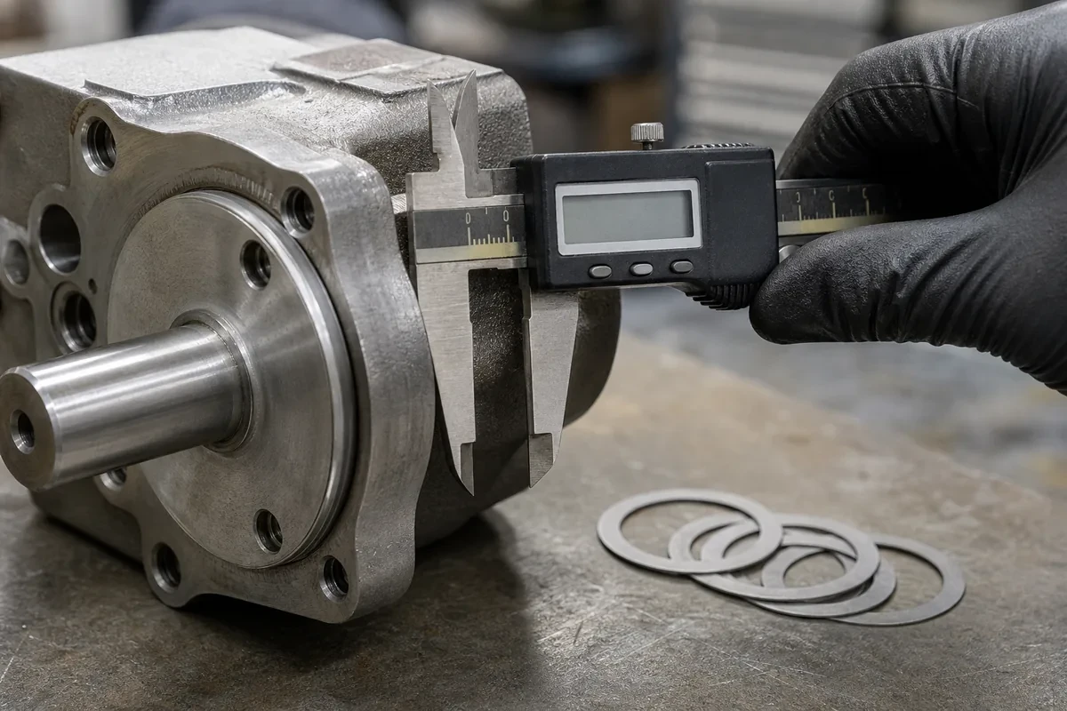
A tolerance stack-up is the arithmetic that answers a simple question: if every part in this assembly is at the worst allowable end of its tolerance, will it still go together? It is the least glamorous part of mechanical design and one of the most valuable, because it is where "each part passed inspection" turns into "the assembly does not fit".
This guide walks through a complete worked example with real numbers, compares worst-case and statistical methods, and shows which design changes actually reduce the stack.
| Method | Formula | Assumption | When to use |
|---|---|---|---|
| Worst case (WC) | Total = Σ individual tolerances | Every part is simultaneously at its limit | Safety-critical, low volume, few suppliers |
| Root sum square (RSS) | Total = √(Σ tᵢ²) | Variations are independent and normally distributed | High volume, stable process, cost-sensitive |
Worst case is conservative and easy to defend. RSS gives a smaller, more economical number, but only holds if the parts are genuinely independent — the same machine, same setup, same operator batch often violates that. Use worst case for a first article or a low-volume program, and RSS only when you have process data to justify it.
Setup: a steel shaft with a shoulder sits in an aluminum housing bore, and a cover plate clamps against the shoulder. We need a minimum axial clearance of 0.10 mm so the cover always seats on the housing face rather than on the shaft.
Four dimensions contribute to the gap, measured from the housing mounting face to the cover contact face:
| # | Dimension | Nominal | Tolerance | Contribution to gap |
|---|---|---|---|---|
| 1 | Housing bore shoulder depth | 25.00 mm | ±0.10 | + |
| 2 | Shaft shoulder-to-end length | 24.50 mm | ±0.08 | − |
| 3 | Cover plate thickness at contact | 0.30 mm | ±0.05 | − |
| 4 | Gasket compressed thickness | 0.20 mm | ±0.05 | − |
25.00 − 24.50 − 0.30 − 0.20 = 0.00 mm. At nominal, there is no clearance at all. That is already a red flag, but nominal is not what matters.
Take the smallest housing depth and the largest of everything subtracted:
(25.00 − 0.10) − (24.50 + 0.08) − (0.30 + 0.05) − (0.20 + 0.05)
= 24.90 − 24.58 − 0.35 − 0.25 = −0.28 mm
The worst case is interference, not clearance. Total stack = 0.10 + 0.08 + 0.05 + 0.05 = 0.28 mm, and the nominal gap of zero means the entire stack eats into the requirement.
To guarantee 0.10 mm minimum clearance, the nominal gap must be at least 0.10 + 0.28 = 0.38 mm. So the shaft needs to be shortened by 0.38 mm (to 24.12 mm nominal), or the housing depth increased by the same amount, or the tolerances tightened.
√(0.10² + 0.08² + 0.05² + 0.05²) = √(0.0100 + 0.0064 + 0.0025 + 0.0025) = √0.0214 = 0.146 mm
With RSS, a nominal gap of 0.25 mm would give 0.10 mm at roughly 3σ. That is a much cheaper design than the worst-case 0.38 mm — but it accepts a small probability of interference. For a production run of 10,000 units with stable processes, that trade can be reasonable. For ten units going into a safety-critical assembly, it is not.
Three things are worth noticing in this example:
That last point is the usual fix: change the nominal rather than tighten the tolerances. It is almost always cheaper. Our cost reduction guide covers this alongside other quoting levers.
Traditional ± coordinate dimensioning chains tolerances in both directions and accumulates them. GD&T can shorten the chain in two ways:
A hole pattern specified with position Ø0.1 at MMC to a shared datum scheme gains bonus tolerance as the holes grow. In a clearance-fit assembly, this is a formal, inspectable way to allow more variation without risking fit — see our datum selection guide for how to set up the reference frame.
A profile of a surface tolerance controls a whole face relative to the datums in one callout. Replacing five chained ± dimensions with one profile removes four accumulation steps from the stack. This is the single most effective structural change available on complex housings.
Be aware that GD&T does not magically reduce variation — it reduces the number of independent contributors and makes the ones that remain functional. A profile tolerance still needs to be achievable by the process.
RSS is the simplest statistical method. If the assembly has more than six contributors, non-normal distributions (a gasket compression is rarely normal), or a supplier whose process drifts rather than varies randomly, a Monte Carlo simulation is more honest. Feed it the actual distribution of each dimension rather than assuming ± equals 3σ, and report the predicted defect rate rather than a single pass/fail gap.
That level of analysis is standard in automotive and aerospace programs, and it pairs naturally with first article inspection data. Our quality control guide explains which measurements to capture on the first article so the model has real inputs.
The stack-up above starts with a set of existing tolerances and asks whether the assembly fits. In a new design the more useful question is the reverse: given the functional clearance we must guarantee, how much tolerance can each part afford?
Suppose the loop in our example contains four dimensions and the worst-case budget is 0.20 mm. The naive approach is equal allocation — 0.05 mm to each. It is fair, but rarely economical: holding ±0.05 on a milled housing depth is straightforward, while holding ±0.05 on a compressed gasket thickness is close to impossible and would require a controlled-compression assembly procedure.
Equal-precision allocation works better. Assign each dimension a tolerance proportional to what its process can hold cheaply, then verify the sum stays within budget. In practice that means giving the machined features looser values (±0.08, ±0.06) and treating the gasket as a fixed, characterized input rather than a tolerance to be tightened — specify a controlled compressed thickness with a stop, and its variation largely disappears from the loop.
Three rules make allocation predictable:
Document the allocation alongside the stack calculation. When a supplier later asks to loosen a dimension, the answer becomes arithmetic rather than negotiation — and the drawing shows which callouts are genuinely functional. Our tolerances guide covers which values are economical to hold on machined features.
Worst case sums all tolerances and assumes every part is at its limit at once — guaranteed fit, but expensive. RSS takes the square root of the sum of squares and assumes independent normal variation — cheaper, but accepts a small defect probability.
Change the nominal dimension to add clearance, shorten the chain by using a shared datum scheme, or replace chained ± dimensions with a single profile callout. All three are usually cheaper than halving a tolerance.
It can. True position at MMC captures bonus tolerance that actually exists in clearance-fit assemblies, and profile controls replace multiple accumulating linear dimensions with one. It reduces the number of contributors rather than the variation itself.
The largest one. In the example above, ±0.10 contributed 36% of the total stack; tightening three ±0.05 items to ±0.02 achieved less than tightening that single dimension.
When parts are not independent — same machine, same setup, same material batch — or when volumes are low, processes are unproven, or the consequence of interference is safety-related. In those cases use worst case.
The arithmetic is not difficult; the discipline is in writing down the loop and refusing to hand-wave the nominal gap. If you share the assembly model at RFQ stage, a supplier can often spot an unclosed stack before any metal is cut — see our RFQ template guide for what to include.
